Sample radiation therapy optimization
In this demo, we illustrate a few simple examples of plan optimization for radiation therapy. We start by importing the needed packages:
In [1]:
%matplotlib inline
import matplotlib.pyplot as plt
from therapy_planner.interface import PlannerInterface
import numpy as np
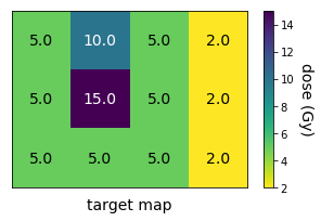
The following is an example input file for dose delivery optimization
with therapy_planner. It lists the target, minimum, and maximum
doses (Gy) to be delivered at each \(1\) cm\(^2\) cell of the
irradiated region.
In [2]:
with open("dose_4x3.map", 'r') as f:
    print(f.read())
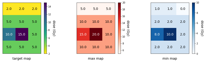
# Target Map
2, 2, 2
5, 5, 5
10, 15, 5
5, 5, 5

# Max Map
5, 5, 5
10, 10, 10
15, 20, 10
10, 10, 10

# Min Map
1, 1, 0
2, 2, 2
8, 10, 2
2, 2, 2
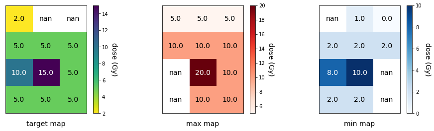
The user begins by creating a plan through the PlannerInterface
Class initialized with an input dose map file. Here we get the target,
max, and min maps, and visualize the specified doses.
In [3]:
m = 4
n = 3
plan = PlannerInterface("dose_4x3.map")
maps = plan.get_maps()

fig, axes = plt.subplots(1,3,figsize=(16,4))
cmaps = ["viridis_r", "Reds", "Blues"]
for key, ax, cmap in zip(maps.keys(),axes.flat,cmaps):
    plan.plot_map(key, ax, cmap)
plt.show()
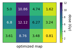
Next we run the optimize method of the PlannerInterface Class
outlined in the interface module. The required input is the incident
beam intensity, in mW, of the horizontal and vertical beams (assumed
equal), which is used to optimize two quantities: 1. horizontal and
vertical beam exposure times 2. sequence of collimator apertures for
each beam, adjusted over the course of exposure, to tune the amount of
radiation delivered to specific regions.
By setting bounds=True, we include a penalty term for optimized dose
maps whose values lie outside of the provided minimum and maximum
values. The smoothness (default 1) adjusts how strongly those bounds are
enforced; a lower smoothness more strictly enforces these constraints,
but is also more prone to numerical instability.
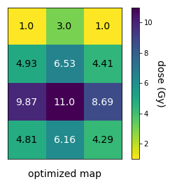
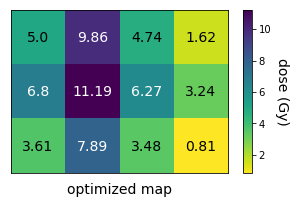
The optimize method computes the optimized dose map and the
horizontal and vertical beam objects, whose attributes include the beam
intensity and exposure time, intermediate “beamlets” used to solve for
the collimator apertures, and the sequence of left and right collimator
positions. In addition, the print_summary() method prints a summary
of several useful aspects of the plan.
In [4]:
plan.optimize(intensity=1., bounds=True, smoothness=0.5)
plan.plot_map("optimized")

plan.print_summary()
Minimum found.
Time Elapsed: 0.7560 sec.
Horizontal beam intensity: 1.00 mW/cm^2
Horizontal beam exposure time: 9 sec.
Vertical beam intensity: 1.00 mW/cm^2
Vertical beam exposure time: 3 sec.
Total accumulated dose: 65.69 Gy
Average dose per unit area: 5.47 Gy/cm^2
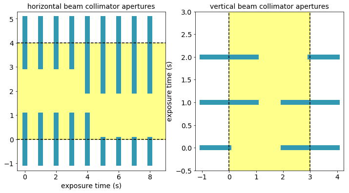
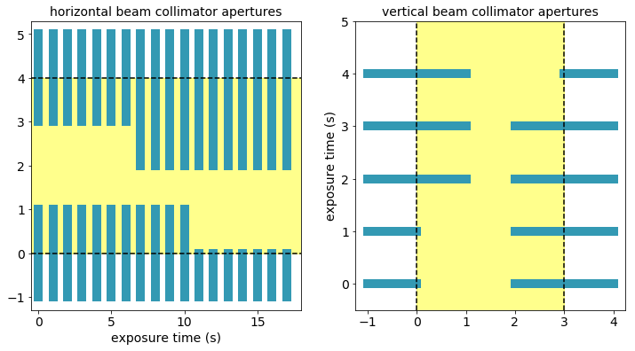
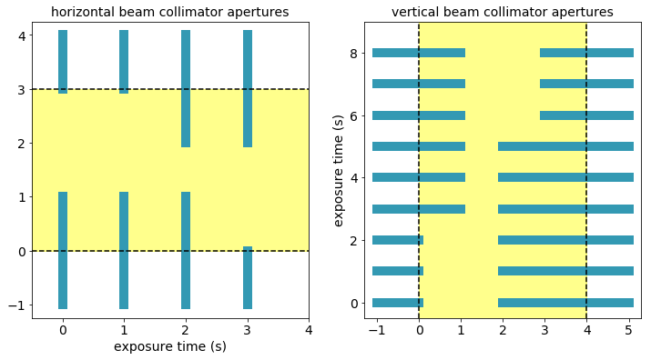
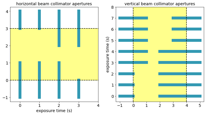
Below we visualize the adjustment of the collimator apertures over the course of the exposure time to achieve the desired dose. For example, we can observe that the second slot of the vertical beam collimator remains exposed to radiation over the full exposure time, and is in fact the column which receives the highest dose.
In [5]:
plan.plot_collimators()
We can also observe the effect of decreasing the intensity, which permits a longer exposure time for dose delivery.
In [6]:
plan.optimize(intensity=0.5, bounds=True, smoothness=0.5)
plan.plot_map("optimized")

plan.print_summary()
Minimum found.
Time Elapsed: 0.8030 sec.
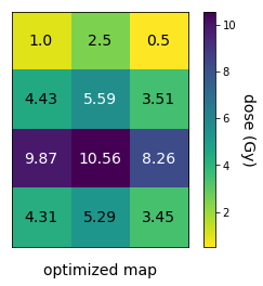
Horizontal beam intensity: 0.50 mW/cm^2
Horizontal beam exposure time: 18 sec.
Vertical beam intensity: 0.50 mW/cm^2
Vertical beam exposure time: 5 sec.
Total accumulated dose: 59.28 Gy
Average dose per unit area: 4.94 Gy/cm^2
In [7]:
plan.plot_collimators()
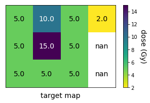
We can also allow rotation of the maps in order to achieve minimum cost
among all 4 rotations, by setting allow_rotation to True.
In [8]:
plan.optimize(intensity=1., bounds=True, allow_rotation=True)
plan.plot_map("target")
plan.plot_map("optimized")
plan.print_summary()
plan.plot_collimators()
Optimize for rotation: 0 degrees
Minimum found.
Negative beamlet value detected. Suggestion: Adjust the smoothness.
Optimize for rotation: 90 degrees
Minimum found.
Negative beamlet value detected. Suggestion: Adjust the smoothness.
Optimize for rotation: 180 degrees
Minimum found.
Optimize for rotation: 270 degrees
Minimum found.
Found best rotation (counter-clockwise): 270 degrees
Time Elapsed: 2.3460 sec.
Maps are rotated for optimality.
Optimal rotation (counter-clockwise): 270 degrees
Horizontal beam intensity: 1.00 mW/cm^2
Horizontal beam exposure time: 4 sec.
Vertical beam intensity: 1.00 mW/cm^2
Vertical beam exposure time: 9 sec.
Total accumulated dose: 67.31 Gy
Average dose per unit area: 5.61 Gy/cm^2
The input maps may also have missing values, as shown in the modified
example below. The optimize routine will obtain the best solution
using only the available constraints.
In [9]:
plan = PlannerInterface("dose_4x3_NaN.map")
maps = plan.get_maps()

fig, axes = plt.subplots(1,3,figsize=(16,4))
cmaps = ["viridis_r", "Reds", "Blues"]
for key, ax, cmap in zip(maps.keys(),axes.flat,cmaps):
    plan.plot_map(key, ax, cmap)
plt.show()
In [10]:
plan.optimize(intensity=1., bounds=True, allow_rotation=True)
plan.plot_map("target")
plan.plot_map("optimized")
plan.print_summary()
plan.plot_collimators()
Optimize for rotation: 0 degrees
Minimum found.
Optimize for rotation: 90 degrees
Minimum found.
Negative beamlet value detected. Suggestion: Adjust the smoothness.
Optimize for rotation: 180 degrees
Minimum found.
Optimize for rotation: 270 degrees
Minimum found.
Found best rotation (counter-clockwise): 270 degrees
Time Elapsed: 1.9418 sec.
Maps are rotated for optimality.
Optimal rotation (counter-clockwise): 270 degrees
Horizontal beam intensity: 1.00 mW/cm^2
Horizontal beam exposure time: 4 sec.
Vertical beam intensity: 1.00 mW/cm^2
Vertical beam exposure time: 8 sec.
Total accumulated dose: 64.51 Gy
Average dose per unit area: 5.38 Gy/cm^2
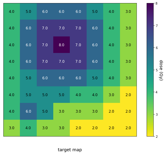
As a final example, we next test a larger map:
In [11]:
m = 8
n = 8
plan = PlannerInterface("dose_8x8.map")
plan.plot_map("target",fontsize=12)
In [12]:
plan.optimize(intensity=0.2, bounds=True)
Minimum found.
Time Elapsed: 28.8361 sec.
In [13]:
plan.plot_map("optimized", fontsize=12)
plan.print_summary()
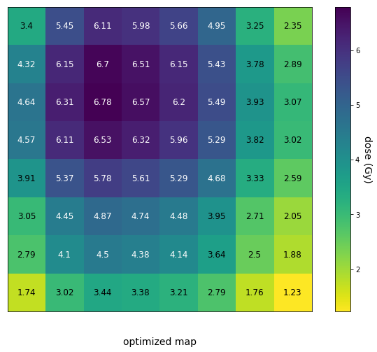
Horizontal beam intensity: 0.20 mW/cm^2
Horizontal beam exposure time: 18 sec.
Vertical beam intensity: 0.20 mW/cm^2
Vertical beam exposure time: 21 sec.
Total accumulated dose: 279.07 Gy
Average dose per unit area: 4.36 Gy/cm^2
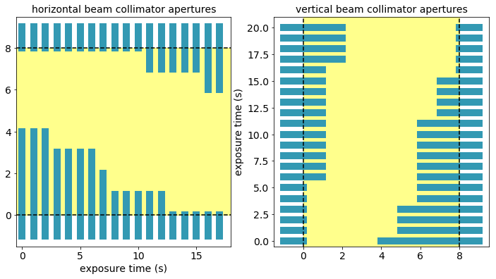
In [14]:
plan.plot_collimators()
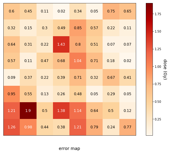
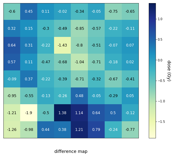
We can also plot the difference between the optimized dose map and the target map to highlight over and underdosed regions, as well as the error (magnitude of the difference plot).
In [15]:
plan.plot_map("difference", cmap='YlGnBu', fontsize=12)
In [16]:
plan.plot_map("error", cmap='OrRd', fontsize=12)