Special functions

In the following demo, we demonstrate use cases of two functions that may be imported from the gradpy.math module: Sin and Exp, as examples of how the derivative of expressions incorporating these special functions may be obtained.

%matplotlib inline
import numpy as np
import matplotlib.pyplot as plt
from gradpy.autodiff import Var
from gradpy.math import Sin, Exp

Sin function

We begin by defining a single-variable function

\[f(x) = 2\sin\left(x\right)\]

in terms of \(x\), whose value is uninitialized.

x = Var()
f = 2*Sin(x)

We compute the value of \(f\) and its derivative with respect to \(x\) at selected points on the interval \([0,8\pi]\) by assigning variable \(x\) its value at each point, evaluating the value attribute of \(f\), and computing the derivative with the der method.

xval = np.arange(0,8*np.pi+.01,0.01)
fval = np.zeros(len(xval))
fder = np.zeros(len(xval))
for i, val in enumerate(xval):
    x.set_value(val)
    fval[i] = f.value
    fder[i] = f.der(x)

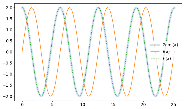
Finally we plot \(f\) and its derivative, along with the analytical solution \(f^{\prime}(x) = 2\cos\left(x\right)\) for comparison.

fig, ax = plt.subplots(1,1,figsize=(10,6))
ax.plot(xval, 2*np.cos(xval), linewidth=7, alpha=0.2, label='$2\\cos(x)$')
ax.plot(xval, fval, label='$f(x)$')
ax.plot(xval, fder, linestyle='dashed', label='$f^{\\prime}(x)$')

plt.xticks(size=14)
plt.yticks(size=14)
plt.legend(fontsize=14)
plt.show()

Exp function

Next we look at a common mathematical model involving the exponential - the logistic equation for population growth:

\[N(t) = \dfrac{K}{1+\left(\dfrac{K}{N_i}-1\right)e^{-rt}}\]

where \(N(t)\) is the population at time \(t\),

\(r\) is the rate of maximum population growth,

\(K\) is the carrying capacity, and

\(N_i\) is the initial population at \(t=0\).

As we will seek the derivative of the model with respect to \(t\), we use the autodiff.math module’s Exp function when defining the logistic_growth function:

def logistic_growth(t,r,K,Ni):
    # r is the rate of maximum population growth
    # K is the carrying capacity
    # Ni is the initial population
    # returns the population at time t
    fac = (K/Ni-1)
    return K/(1+fac*Exp(-r*t))

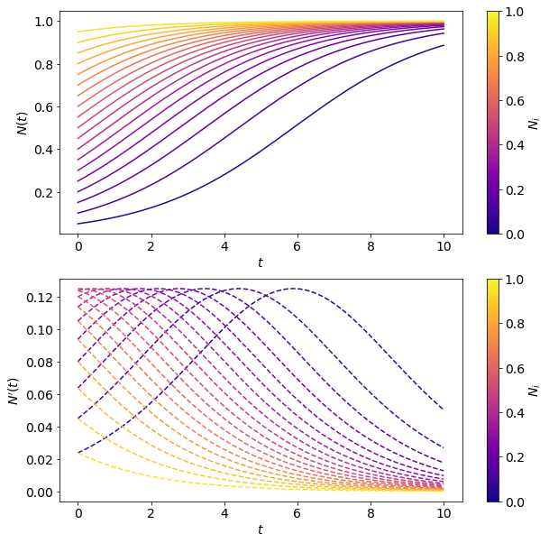
We track the evolution of a population with a maximum growth rate \(r=0.5\), carrying capacity \(K\) normalized to 1, and varied initial population sizes \(N_i \in [0.05,0.95]\), on a time interval \(t = [0,10]\). The variable \(t\) is an autodiff variable, so we can compute the derivative of \(N\) with respect to \(t\) corresponding to each \(N_i\) and timestep.

t = Var()
r = 0.5
K = 1
Ns = np.arange(0.05,1,0.05)

tval = np.arange(0,10.01,0.01)
Nval = np.zeros((len(Ns),len(tval)))
Nder = np.zeros((len(Ns),len(tval)))

for i,Ni in enumerate(Ns):
    N = logistic_growth(t,r,K,Ni)
    for j, val in enumerate(tval):
        t.set_value(val)
        Nval[i,j] = N.value
        Nder[i,j] = N.der(t)

Finally, we visualize the results below.

fig, (ax1,ax2) = plt.subplots(2,1,figsize=(10,10))
cmap = plt.cm.get_cmap('plasma')
for i,Ni in enumerate(Ns):
    col = cmap(Ni)
    ax1.plot(tval, Nval[i,:], color=col)
    ax2.plot(tval, Nder[i,:], color=col, linestyle='dashed')

# axes
ax1.set_xlabel('$t$',size=14)
ax1.set_ylabel('$N(t)$',size=14)
ax1.tick_params(labelsize=14)
ax2.set_xlabel('$t$',size=14)
ax2.set_ylabel('$N^{\\prime}(t)$',size=14)
ax2.tick_params(labelsize=14)

# colorbars
sm = plt.cm.ScalarMappable(cmap=cmap)
sm.set_array([])
cbar1 = plt.colorbar(sm, ax=ax1)
cbar1.set_label('$N_i$',size=14)
cbar1.ax.tick_params(labelsize=14)
cbar2 = plt.colorbar(sm, ax=ax2)
cbar2.set_label('$N_i$',size=14)
cbar2.ax.tick_params(labelsize=14)

plt.show()